

P1:tensorflow安装
1 | pip install tensorflow |
P2:Hello World——衣服分类
这个例子训练了一个神经网络模型,用于分类衣服图片,比如tshirt和运动鞋。
需要用到tf.keras,它是个用于建立和训练模型的高层次的API
1 | # TensorFlow and tf.keras |
2.2.0
导入Fashion MNIST数据集
1 | fashion_mnist = keras.datasets.fashion_mnist |
导入数据集,返回Numpy数组:
train_images和train_labels数组是训练集。test_images和test_labels数组是测试集。
这些图像是28x28的Numpy数组。可以理解为28x28的像素点,这些像素点在屏幕上显示出来表现为图像。每个像素点的值在0到255之间,表示颜色的深浅。如果你了解颜色的RGB值,那你就明白,所有的颜色都是由不同深浅程度的三种基本色构成,比如白色的RGB为(255.255.255)。标签labels是一个整数数组,范围从0到9。表示10个不同的衣服种类Class。
| Label | Class |
|---|---|
| 0 | T-shirt/top |
| 1 | Trouser |
| 2 | Pullover |
| 3 | Dress |
| 4 | Coat |
| 5 | Sandal |
| 6 | Shirt |
| 7 | Sneaker |
| 8 | Bag |
| 9 | Ankle boot |
这些种类不包括在数据集中,需要单独定义:
1 | class_names = ['T-shirt/top', 'Trouser', 'Pullover', 'Dress', 'Coat', 'Sandal', 'Shirt', 'Sneaker', 'Bag', 'Ankle boot'] |
研究数据
在训练模型之前,先研究这些数据格式。比如在训练集中的六万张图片,每张图片由28x28的像素点表示。
1 | train_images.shape |
(60000, 28, 28)
同时还有六万个与之对应的标签:
1 | len(train_labels) |
60000
每个标签都是一个0到9之间的整数:
1 | train_labels |
array([9, 0, 0, …, 3, 0, 5], dtype=uint8)
还有一万张用于测试的图片:
1 | test_images.shape |
(10000, 28, 28)
一万张训练集的标签:
1 | len(test_labels) |
10000
数据预处理
在训练模型之前,必须先对数据进行预处理。观察第一张图,我们可以看到图片的像素值在0到255之间。
1 | plt.figure() |

将像素值范围缩小为0到1,所以将像素值都除以255:
1 | train_images = train_images / 255.0 |
为了确保数据的正确性,先将训练集的前25个图片显示出来,并且在图片下面展示分类名。
1 | plt.figure(figsize=(10,10)) |

建立模型
建立神经网络需要配置模型层,然后编译模型。
设置层
基本的神经网络模块是层。层会从它们获取的数据里提取图像。它们希望从这些图像里获取有用的信息。
大多数深度学习都是简单层组合在一起。大多数层比如tf.keras.layers.Dense,拥有在训练时学习到的参数。
1 | model = keras.Sequential([ keras.layers.Flatten(input_shape=(28, 28)), keras.layers.Dense(128, activation='relu'), keras.layers.Dense(10)]) |
这个网络的第一层,tf.keras.layers.Flatten,将图像的格式从二维数组(28 * 28像素)转换为一维数组(28 * 28 = 784像素)。可以将这一层看作是将图像中的像素行展开并排列起来。这一层没有参数需要学习;它只是重新格式化数据。
像素被扁平化后,网络由两个tf.keras.层组成。它们是紧密相连或完全相连的神经层。第一致密层有128个节点(或神经元)。第二个(也是最后一个)层返回长度为10的logits数组。每个节点都包含一个评价值,表示当前图像属于这10个类中的一个。
编译模型
在准备训练模型之前,需要进行一些其他设置。 这些是在模型的编译步骤中添加的:
- Loss function——这可以衡量模型在培训期间的准确性。您希望最小化这个函数,以便将模型“引导”到正确的方向。
- Optimizer——这就是模型如何根据它看到的数据和它的损失函数进行更新。
- Metrics——用于监控培训和测试步骤。下面的例子使用了准确率,即正确分类的图像的比例。
1 | model.compile(optimizer='adam', loss=tf.keras.losses.SparseCategoricalCrossentropy(from_logits=True), metrics=['accuracy']) |
训练模型
训练神经网络模型需要以下步骤:
- 输入训练数据到模型中。
- 模型学习关联图像和分类标签。
- 让模型预测测试集。
- 验证预测结果是否和标签匹配。
输入数据到模型中
利用model.fit方法。他能将模型用于拟合训练数据。
1 | model.fit(train_images, train_labels, epochs=10) |
Epoch 1/10
1875/1875 [==============================] - 3s 2ms/step - loss: 0.4978 - accuracy: 0.8248
Epoch 2/10
1875/1875 [==============================] - 3s 2ms/step - loss: 0.3767 - accuracy: 0.8637
Epoch 3/10
1875/1875 [==============================] - 3s 2ms/step - loss: 0.3397 - accuracy: 0.8759
Epoch 4/10
1875/1875 [==============================] - 3s 2ms/step - loss: 0.3138 - accuracy: 0.8854
Epoch 5/10
1875/1875 [==============================] - 3s 2ms/step - loss: 0.2948 - accuracy: 0.8914
Epoch 6/10
1875/1875 [==============================] - 3s 2ms/step - loss: 0.2803 - accuracy: 0.8958
Epoch 7/10
1875/1875 [==============================] - 3s 2ms/step - loss: 0.2678 - accuracy: 0.9006
Epoch 8/10
1875/1875 [==============================] - 3s 2ms/step - loss: 0.2590 - accuracy: 0.9043
Epoch 9/10
1875/1875 [==============================] - 3s 2ms/step - loss: 0.2464 - accuracy: 0.9078
Epoch 10/10
1875/1875 [==============================] - 3s 2ms/step - loss: 0.2402 - accuracy: 0.9099<tensorflow.python.keras.callbacks.History at 0x7fe472eff4a8>
评估准确率
比较模型在测试数据集上的表现:
1 | test_loss, test_acc = model.evaluate(test_images, test_labels, verbose=2) |
313/313 - 1s - loss: 0.3382 - accuracy: 0.8840
Test accuracy: 0.8840000033378601
结果是测试数据集上的准确性比训练数据集上的准确性稍低。训练准确度和测试准确度之间的差距代表过拟合。当机器学习模型在新的、以前没有看到的输入上的表现不如在训练数据上的表现时,就会发生过拟合。过度拟合的模型“记忆”了训练数据集中的噪音和细节,从而对模型在新数据上的性能产生负面影响。有关更多信息,请参见以下内容
预测结果
通过训练模型,你可以使用它来预测某些图像。 模型的线性输出,logits。 附加一个softmax层以将logit转换为更容易解释的概率。
1 | probability_model = tf.keras.Sequential([model, tf.keras.layers.Softmax()]) |
1 | predictions = probability_model.predict(test_images) |
在这里,模型已经预测了测试集中每个图像的标签。 让我们看一下第一个预测:
1 | predictions[0] |
array([1.2275562e-07, 8.9534730e-08, 7.6224147e-09, 1.9726743e-08,
6.1515345e-07, 4.6329503e-03, 4.1164008e-06, 1.5043605e-02,
2.8817641e-07, 9.8031825e-01], dtype=float32)
预测是一个包含10个数字的数组。它们代表了模型的“自信”,即图像对应着10种不同的服装。你可以看到哪个标签的自信度最高:
1 | np.argmax(predictions[0]) |
9
因此,模型最自信的认为这是一个踝靴,或class_names[9]。检查测试标签表明这个分类是正确的:
1 | test_labels[0] |
9
绘制图表,看看10个类预测的全部集合。
1 | def plot_image(i, predictions_array, true_label, img): |
验证预测
通过训练模型,您可以使用它来预测某些图像。
让我们看一下第0张图片,预测和预测数组。 正确的预测标签为蓝色,错误的预测标签为红色。 该数字给出了预测标签的百分比(满分为100)。
1 | i = 0 |

1 | i = 12 |
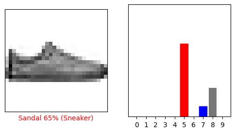
让我们绘制一些带有预测的图像。 请注意,即使非常自信,该模型也可能是错误的。
1 | # Plot the first X test images, their predicted labels, and the true labels. |

使用训练的模型
最后,利用训练好的模型对单幅图像进行预测。
1 | # Grab an image from the test dataset. |
(28, 28)
tf.keras模型经过优化,可以立即对一批或一组示例进行预测。因此,即使使用的是单个图像,也需要将其添加到列表中
1 | # Add the image to a batch where it's the only member. |
(1, 28, 28)
现在为这个图像预测正确的标签
1 | predictions_single = probability_model.predict(img) |
[[2.3256284e-06 5.5768194e-13 9.9955302e-01 3.3701731e-13 4.3444714e-04
3.7890427e-17 1.0105057e-05 4.5671220e-20 8.4883814e-14 9.5599025e-18]]
1 | plot_value_array(1, predictions_single[0], test_labels)_ = plt.xticks(range(10), class_names, rotation=45) |

keras.Model.predict返回列表的列表-数据批次中每个图像的列表。 批量获取我们(唯一)图像的预测:
1 | np.argmax(predictions_single[0]) |
2
这个模型预测了一个标签。
本指南使用Fashion MNIST数据集,该数据集包含10个类别中的70,000张灰度图像。这些图像以低分辨率(28×28像素)显示了衣服的单个物品,如图所示
![]()
Fashion MNIST旨在替代经典MNIST数据集,通常被用作计算机视觉机器学习程序的“ Hello,World”。 MNIST数据集包含手写数字(0、1、2等)的图像,格式与您将在此处使用的衣服的格式相同。
本指南将Fashion MNIST用于多种用途,并且因为它比常规MNIST更具挑战性。 两个数据集都相对较小,用于验证算法是否按预期工作。 它们是测试和调试代码的良好起点。
在这里,使用60,000张图像来训练网络,使用10,000张图像来评估网络学习对图像进行分类的准确程度。 您可以直接从TensorFlow访问Fashion MNIST。 直接从TensorFlow导入和加载Fashion MNIST数据:

博客内容遵循 署名-非商业性使用-相同方式共享 4.0 国际 (CC BY-NC-SA 4.0) 协议
本文永久链接是:https://blog.sci.ci/2020/06/17/TensorFlow%E5%AD%A6%E4%B9%A0%E7%AC%94%E8%AE%B0/